ChEA-KG: Human Transcription Factor Regulatory Network with a Knowledge Graph Interactive User Interface

Table of Contents

1. Abstract
2. The ChEA-KG GRN
3. Searching the KG
   1.  Single term search
   2.  Expanded single term search
   3.  Two term search
4. Interacting with the subnetwork using the toolbar
   1.  Adjust network view
   2.  Downloading the network
5. Enrichment analysis with ChEA-KG
   1.  Performing a query
   2.  Preparing an example
   3.  Filtering the results
   4.  Viewing results in a table or bar chart
6. User Data
7. API
   1.  Analyze a gene set
   2.  View added gene set
   3.  Get enriched subnetwork

Abstract

Gene expression is controlled by transcription factors that selectively bind to DNA to regulate mRNA expression of all human genes. Transcription factors control the expression of other transcription factors, forming a complex gene regulatory network (GRN) with switches, feedback loops, and other regulatory motifs. Many experimental methods and computational tools have been developed to reconstruct GRNs in-silico. Here we present a different approach to reconstruct the human GRN. By submitting thousands of gene sets from the RummaGEO resource for transcription factor enrichment analysis with ChEA3, we are able to distill signed and directed edges that connect all human transcription factors to construct a high quality human GRN. The GRN has 130,793 signed and directed edges between 703 source and 1,543 target transcription factors. The network is made accessible via an interactive web-based application called ChEA-KG. ChEA-KG enables users to query the GRN by searching for single or pairs of transcription factors, as well as by submitting gene sets to perform transcription factor enrichment analysis with ChEA3 and then place the enriched transcription factors in context of ChEA-KG. To demonstrate the utility of ChEA-KG, we systematically identified transcription factor subnetworks that regulate differentially expressed genes in tumors from ten cancer types, and 69 subtypes, profiled by the Clinical Proteomic Tumor Analysis Consortium (CPTAC).

The ChEA-KG GRN

ChEA-KG visualizes a human GRN that connects 1,553 transcription factors (TFs) with signed, directed edges that indicate up- or down-regulatory relationships between TFs. There are 63,375 upregulated edges and 67,418 downregulated edges in the GRN. The network is constructed by inputting 171,441 human gene sets from RummaGEO into ChEA3 for enrichment analysis. For each gene set, edges are identified between each enriched TF, which serves as the source node, and the TFs in the gene set, which become the targets. The final ChEA-KG network is filtered by edge significance using a z-test and a p-value threshold of (p < 0.01).

Nodes

There are 1,554 nodes representing TFs that are found to be highly enriched for any RummaGEO gene set based on the 1,632 TFs cataloged by the ChEA3 primary libraries. Each node is associated with an ID, a label, and a URI that points to the NCBI gene page for that TF.

Edges

Edges in the GRN indicate regulatory relationships between source and target TFs, determined using enrichment analysis with ChEA3. There are two types of edges (Fig. 1).
1 - Red plungers indicate downregulation (inhibition).
2 - Green arrows indicate upregulation (activation).

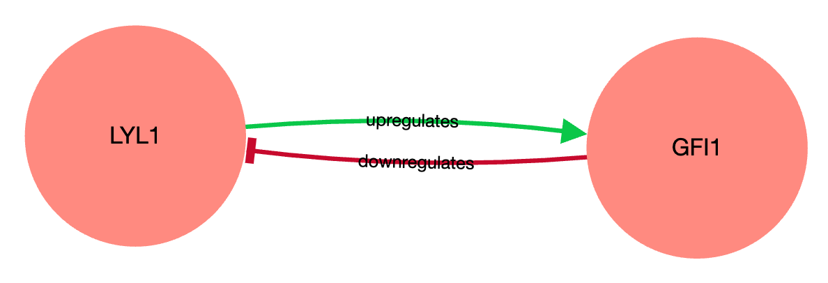
Fig. 1. ChEA-KG subnetwork consists of two TFs connected with two reciprocal edges, denoting LYL1 upregulation of GFI1, and GFI downregulation of LYL1.

 

Searching the KG

The ChEA-KG search page enables users to query specific subnetworks of the GRN. The search page has three key features: the search panel, the network view window, and a toolbar. The search panel provides options to customize the search query, the network view window displays the results, and the toolbar provides buttons to interact with the results. The following sections describe how to use these features.

Single term search

To perform a single-term search, start typing the name of a valid Entrez gene symbol of a TF into the "Start with" field (Fig. 2). If the TF exists in the ChEA-KG network, it will show up in the autocomplete drop-down menu. To perform the search, click on the TF name in the menu. Alternatively, you can click on one of the two example TFs under "Example". A subnetwork displaying the relationships between the search TF and its immediate neighbors will be displayed.

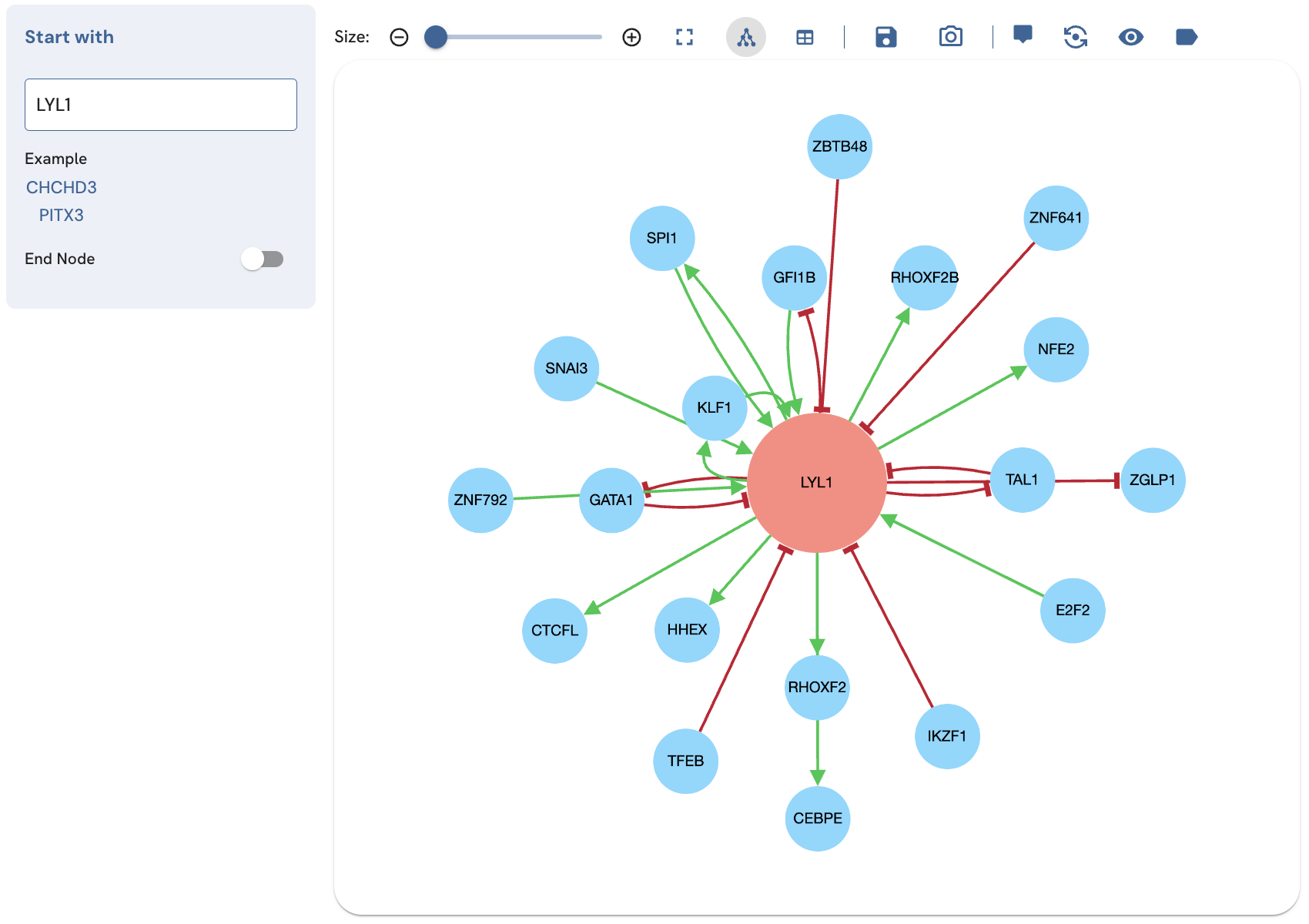
Fig. 2. Subnetwork produced by a single-term search for LYL1.

Expanded single term search

The single term search displays a subnetwork centered around a specific TF while the expanded single term search shows more in depth interactions centered on the same TF. To perform an expanded search of a single TF, input the Entrez gene symbol of the search TF into the "Start with" field, and click on its name in the autocomplete drop-down menu. Next, toggle the "End Node" switch on (Fig. 3). Leave the "End with" field blank. Control the size of the subnetwork using the slider above the network view.

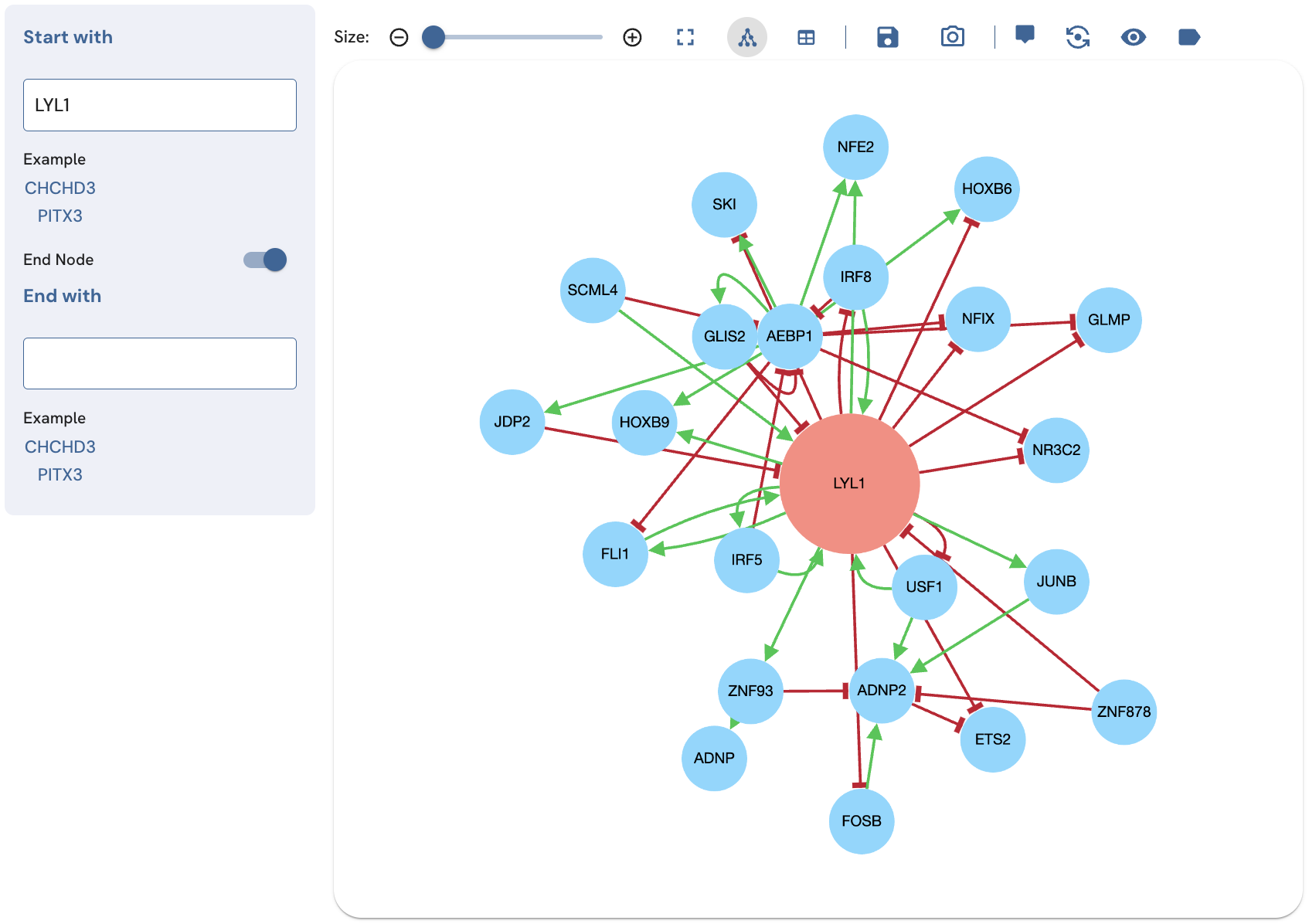
Fig. 3. An expanded LYL1 subnetwork produced by toggling the "End node" switch on and leaving the text box for the end node blank.

Two term search

The two-term search displays the shortest path between two TFs (Fig. 4). In the case where there is a tie for the shortest paths of the same length, all paths of that length will be displayed. To perform the search, enter a starting TF in the "Start with" textbox. Select its name from the autocomplete drop-down menu. Toggle the "End node" switch on, then input a desired end TF in the "End with" field.

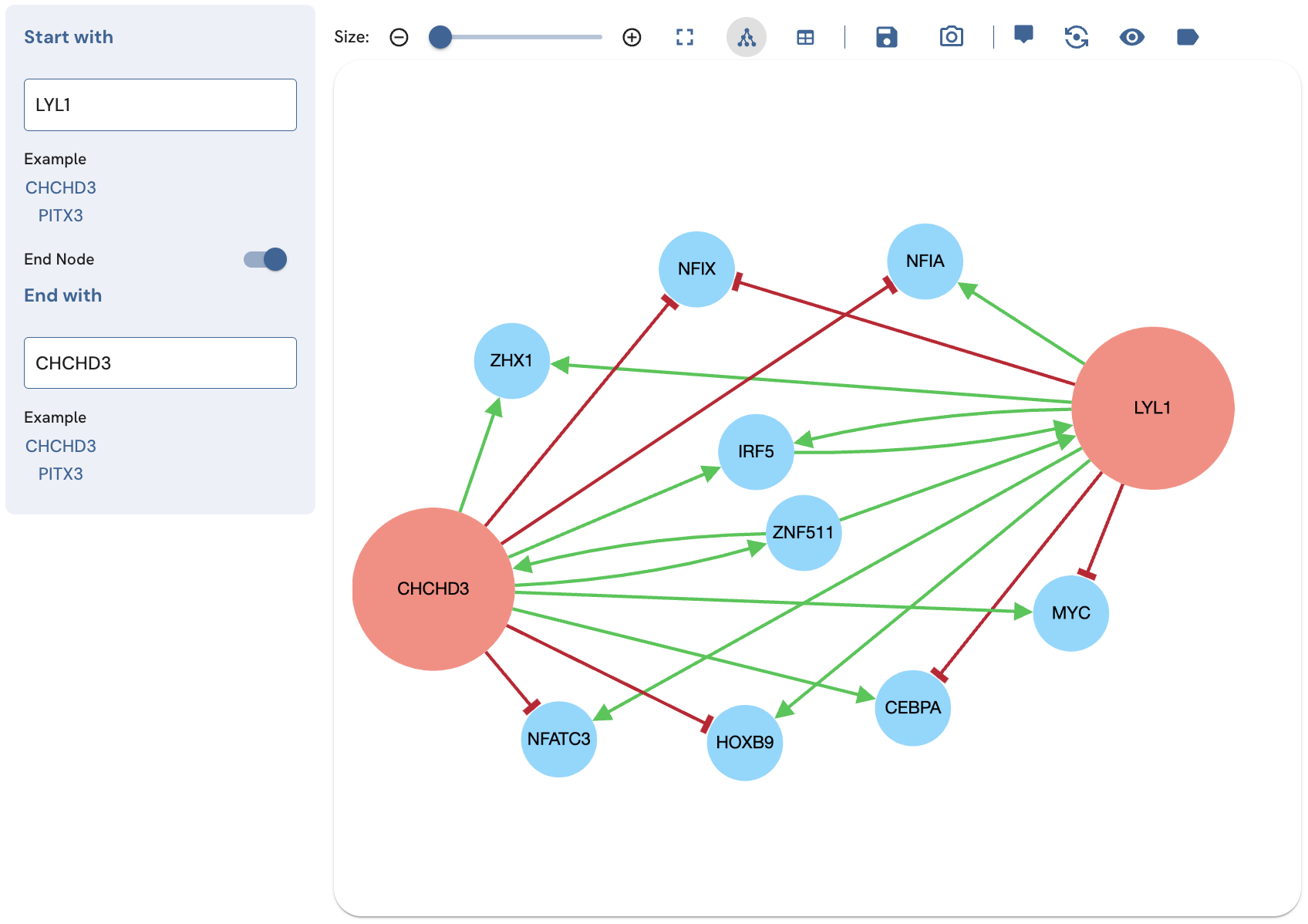
Fig. 4. Fig. 4. Subnetwork produced by a two-term search for finding paths that connect the TFs LYL1 and CHCHDC3. The subnetwork size has been limited to 11, using the slider above the network view.

 

Interacting with the subnetwork using the toolbar

Basic navigation such as zooming in and out, and highlighting nodes and edges are accomplished with the mouse. The toolbar above the network view provides several buttons for additional ways to interact with the subnetwork. From left to right, these tools are Size, Full-screen, Network View, Table View, Save Subnetwork, Download Subnetwork as an Image File, Show Tooltip, Switch Graph Layout, Show Edge Labels, and Show Legend.

 

Adjust the network view

Basic navigation
To rearrange individual network nodes, click on a node and drag it. Use the mouse wheel to zoom in and out. To emphasize a TF and its edges, hover over the TF node with the mouse pointer. Click on the TF to highlight its edges (Fig. 5). Click and drag the whitespace to move the entire subnetwork and pan.

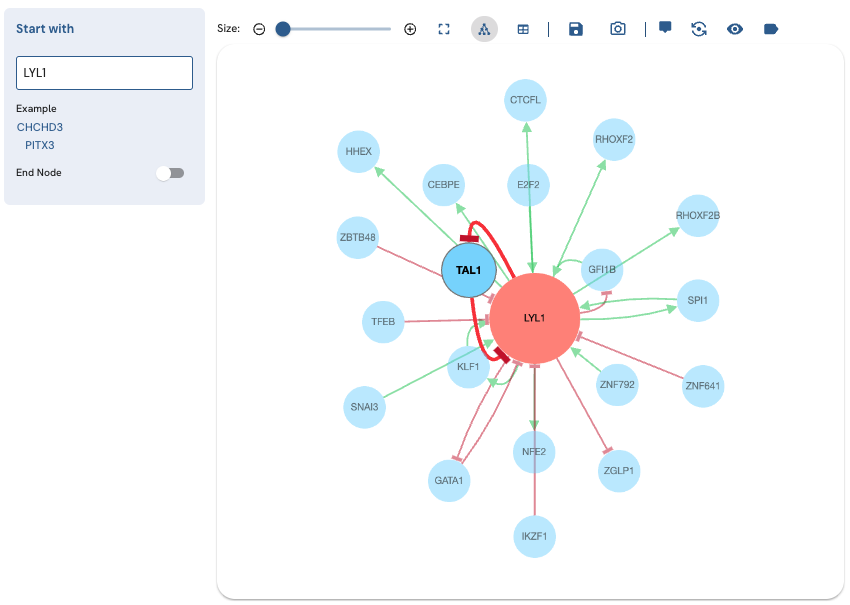
Fig. 5. Highlight a TF and its edges by clicking on it.

 

Adjusting the subnetwork size
Adjust the size of the subnetwork with the slider to limit the number of relationships displayed (Fig. 6). This adds or subtracts edges for the subnetwork. Edges are prioritized based on their z-score. Relationships are prioritized based on their z-score. Z-scores are calculated from expected counts generated by randomly shuffling the network.

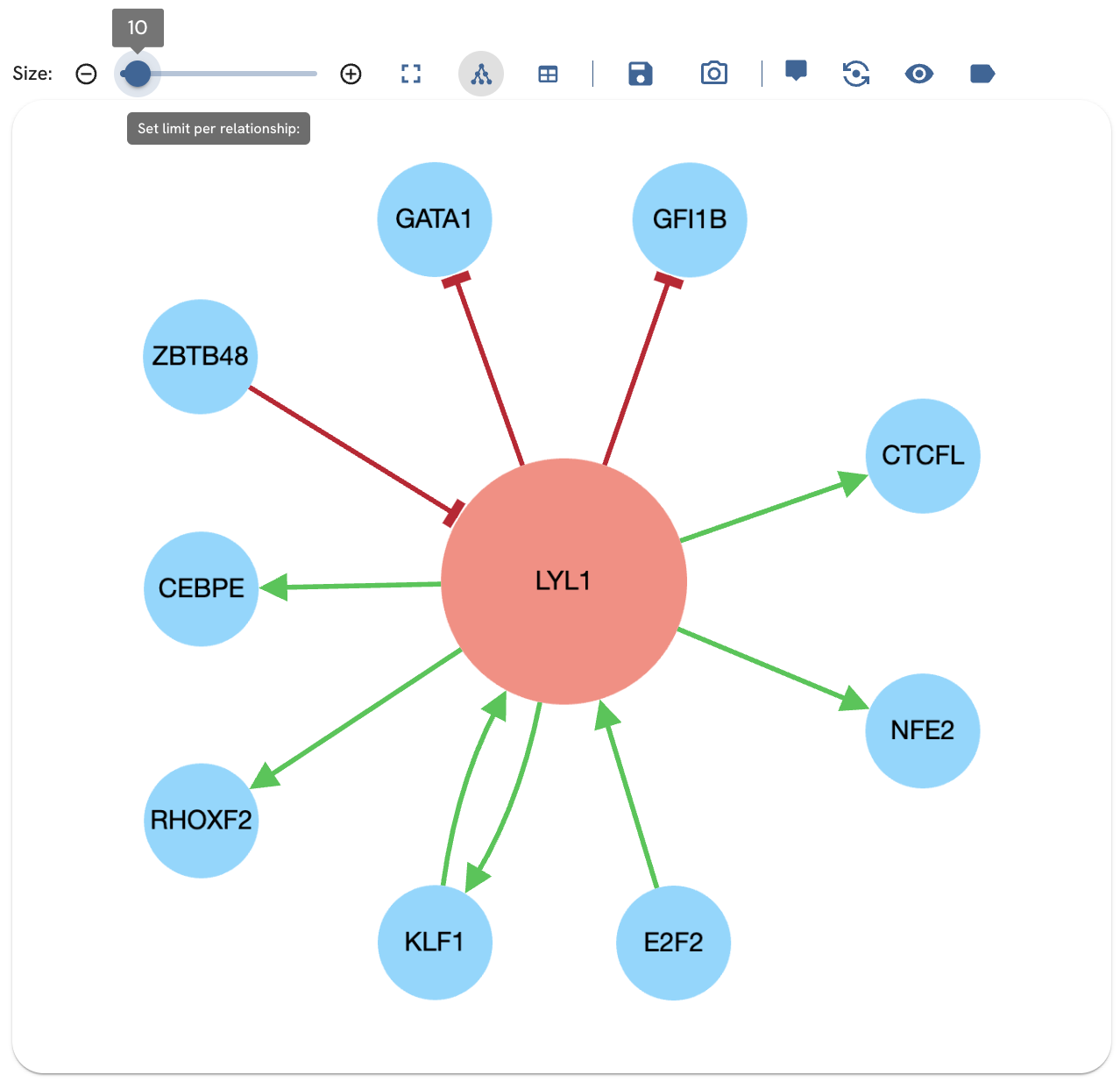
Fig. 6. Adjusting the slider changes the number of edges.

Full screen mode
Clicking on the full-screen button displays the search panel, network view, and toolbar in full-screen.

Enabling the tooltip feature
The tooltip is used to show more information about a TF in the subnetwork. The tooltip lists the ID, label, and URI of the TF. You should be able to see the ID, label, and URI of a TF when mouse hovering over it (Fig. 7).

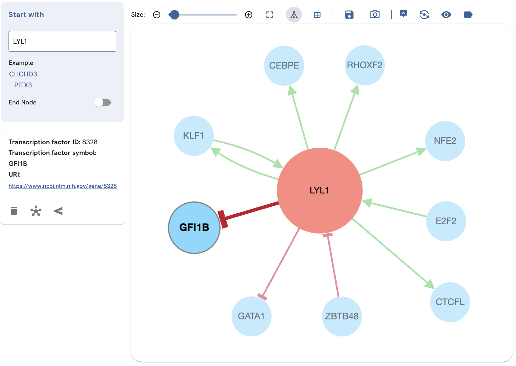
Fig. 7. Enabling the tooltip displays the node ID, label, and URI for each TF that is clicked or hovered over.

Deleting or expanding a TF
The tooltip also provides options to add additional edges for the selected TF (expand), and invoke a single-term search for that TF in a new page (open node in a new page) (Fig. 8). In the single-term search and expanded single-term search, the tooltip also provides the option to delete the TF from the subnetwork (Fig. 9). To use these options, with the tooltip enabled, click on the TF to view its tooltip. Click "delete", "expand", or "open node in a new page" to perform these actions.

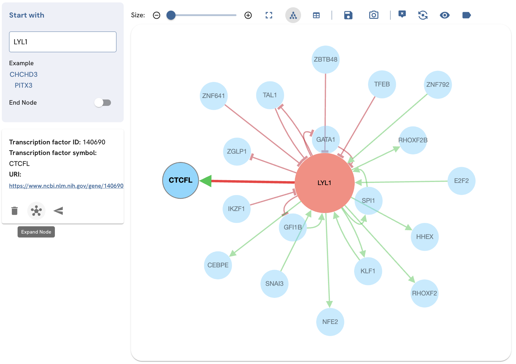
Fig. 8A. Expanding CTCFL by clicking the expand icon.

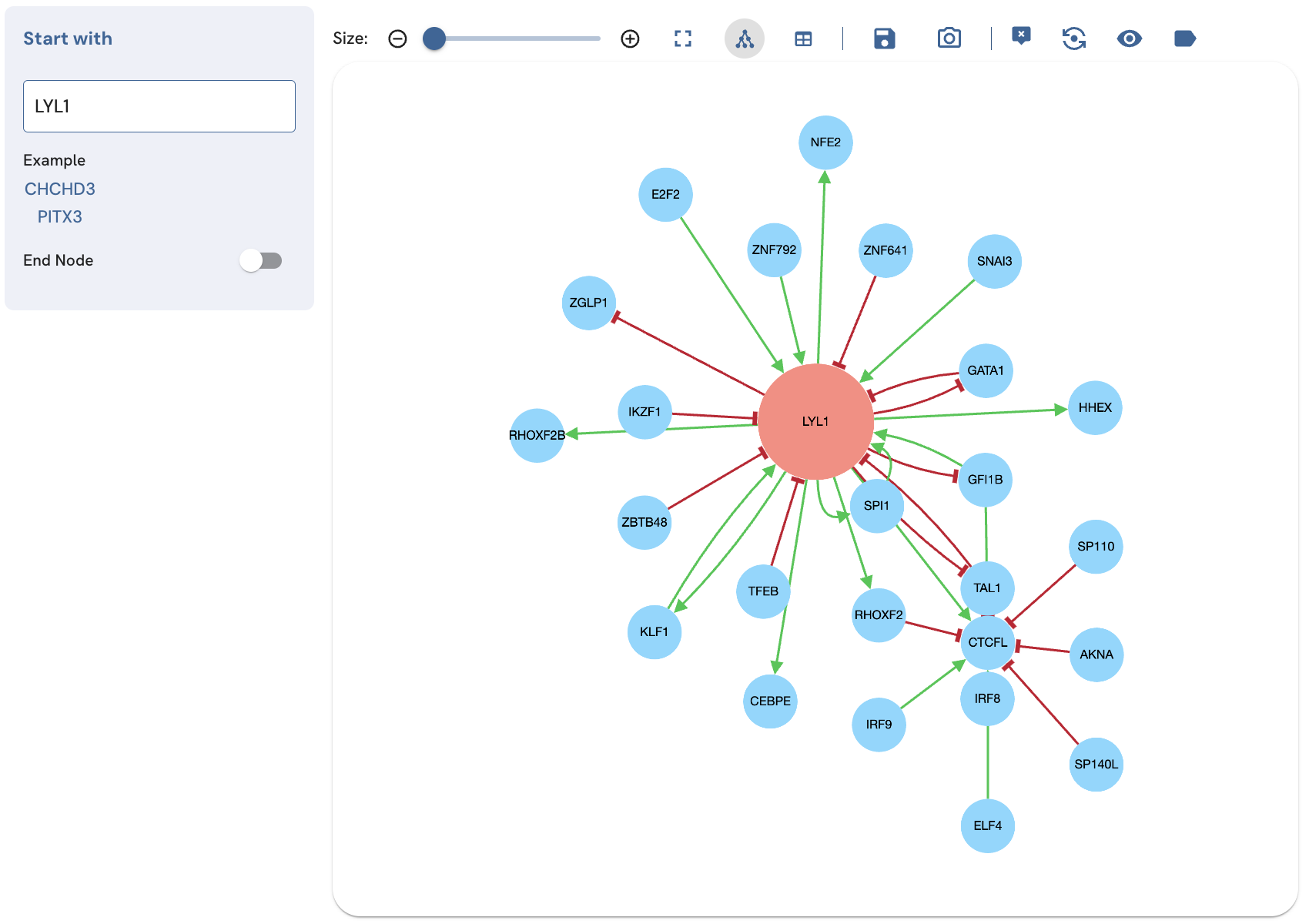
Fig. 8B. Expanding the CTCFL TF by clicking expand displays additional relationships involving CTCFL.

 

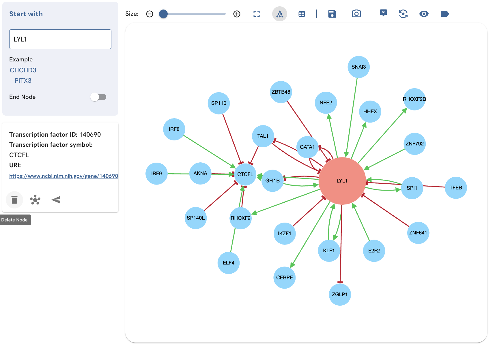
Fig. 9A. Deleting CTCFL by clicking the delete icon.

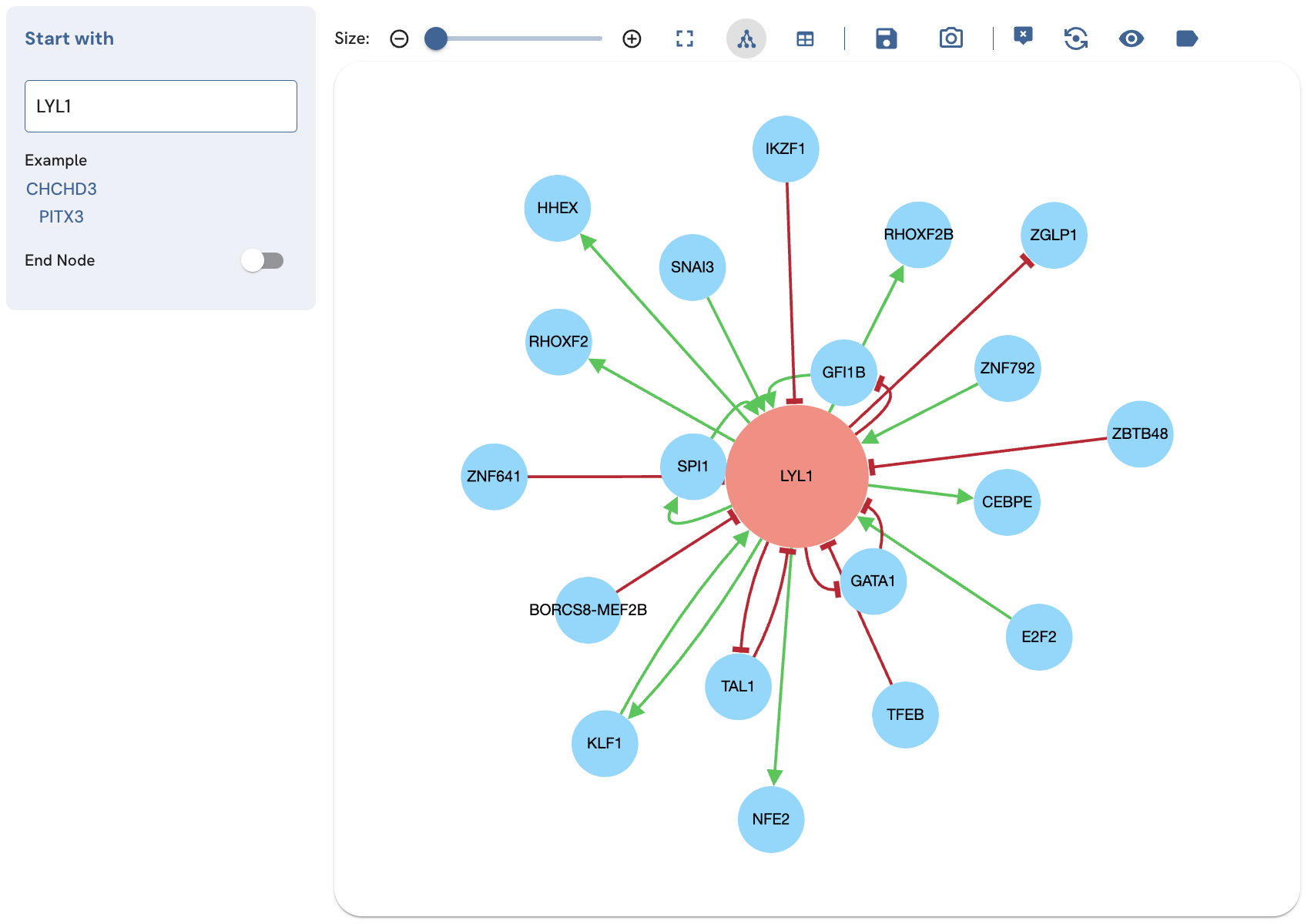
Fig. 9B. Removing CTCFL by clicking the delete icon removes the CTCFL and edges.

Subnetwork and table views
In addition to the subnetwork view, there is also the option to view the subnetwork as a table. To change between the subnetwork and table views, click on their respective buttons (Fig. 10). Three tables are produced, one for the nodes, one for the upregulation edges, and one for downregulation edges. The tables contain the following fields:
      - Nodes: TF ID, symbol, and URI
      - Edges: Source, relation, target, Z score, p-value
Individual entries can be searched by entering a search term into the "Search Results" field. The table can be exported as a CSV file or printed using the "Export" button to the right of the search bar. Clicking on any of the header titles sorts the table according to that field. Adjusting the number of results displayed adds more entries.

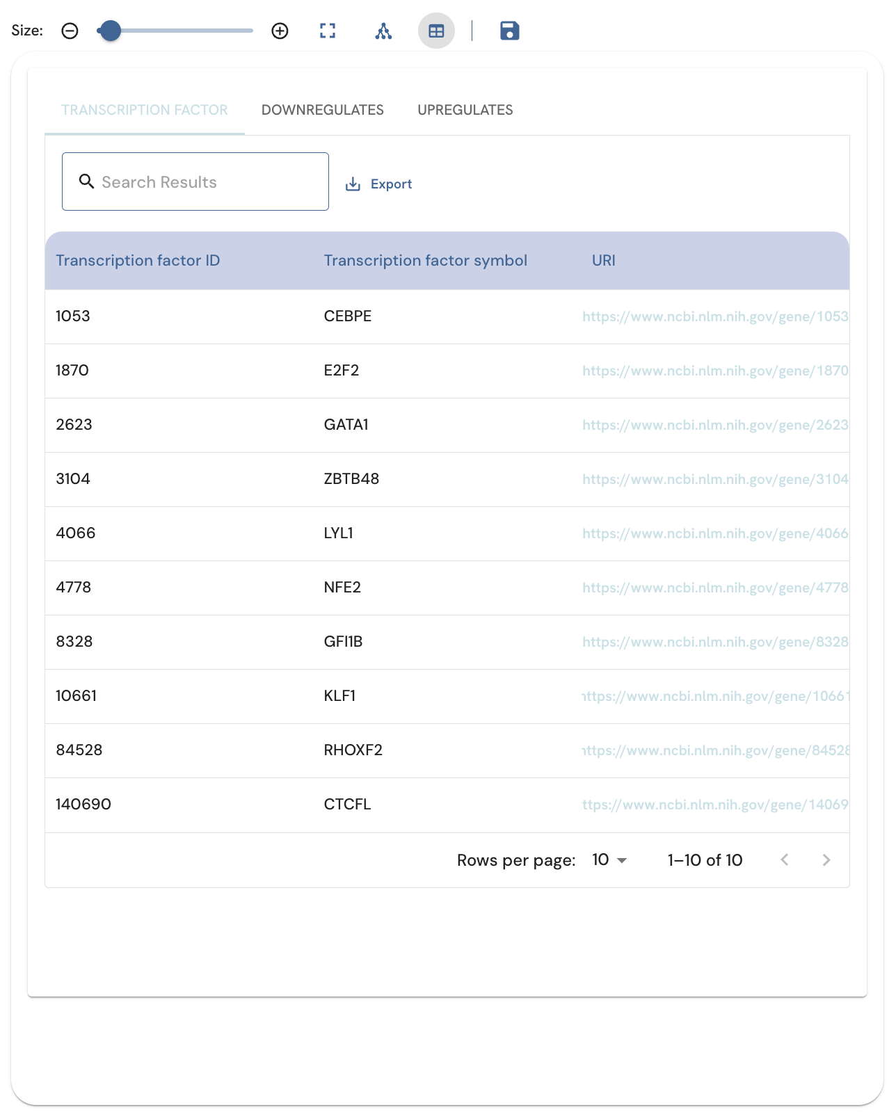
Fig. 10. Viewing the subnetwork as a table with the Table View button.

Switching to the graph layout
The subnetwork view provides three graph layouts. These are 1) force-directed (emphasizes clustering), 2) geometric (organizes nodes into a circle, emphasizing density), and hierarchical (emphasizing the hierarchical structure of the subnetwork). More information about these graph layout algorithms is available on the Cytoscape blog. Switching between the graph layouts can be done by clicking on the Graph Layout button, and then clicking on the name of the desired layout (Fig. 11).

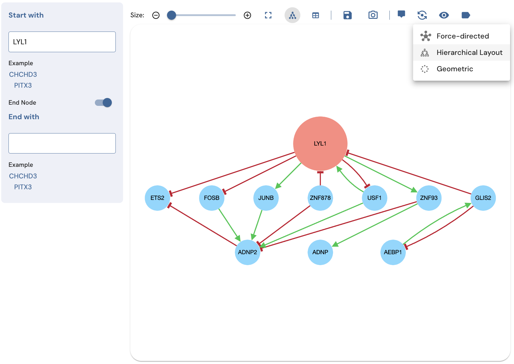
Fig. 11. Example from a hierarchical layout using the Graph Layout button.

Showing the edge labels
To display the edge labels ("upregulates" and "downregulates") on the subnetwork edges, click on the Edge Labels button (Fig. 12).

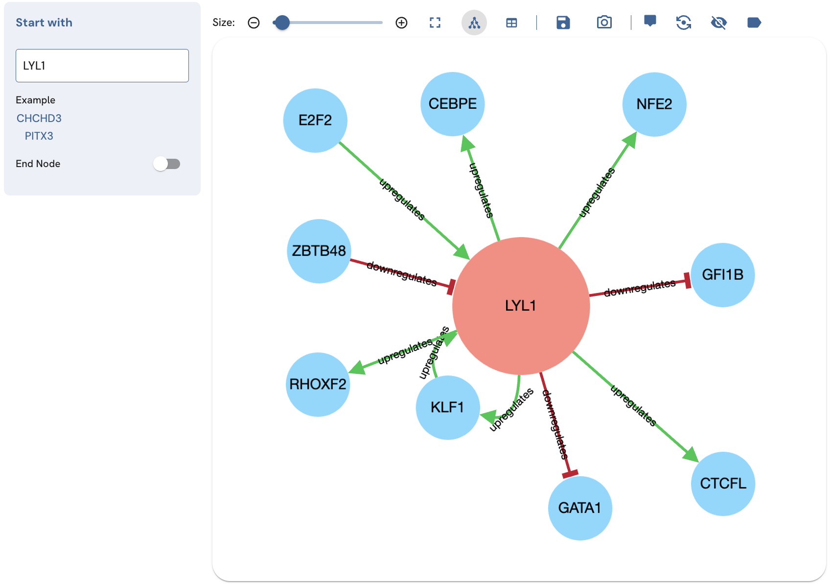
Fig. 12. Display the edge labels using the Edge Labels button.

Showing the legend
To display a legend describing the node and edge colors, use the “Show Legend” button (Fig. 13). Once clicking the button, an additional tool is added to the toolbar. This button can be used to adjust the size of the legend.

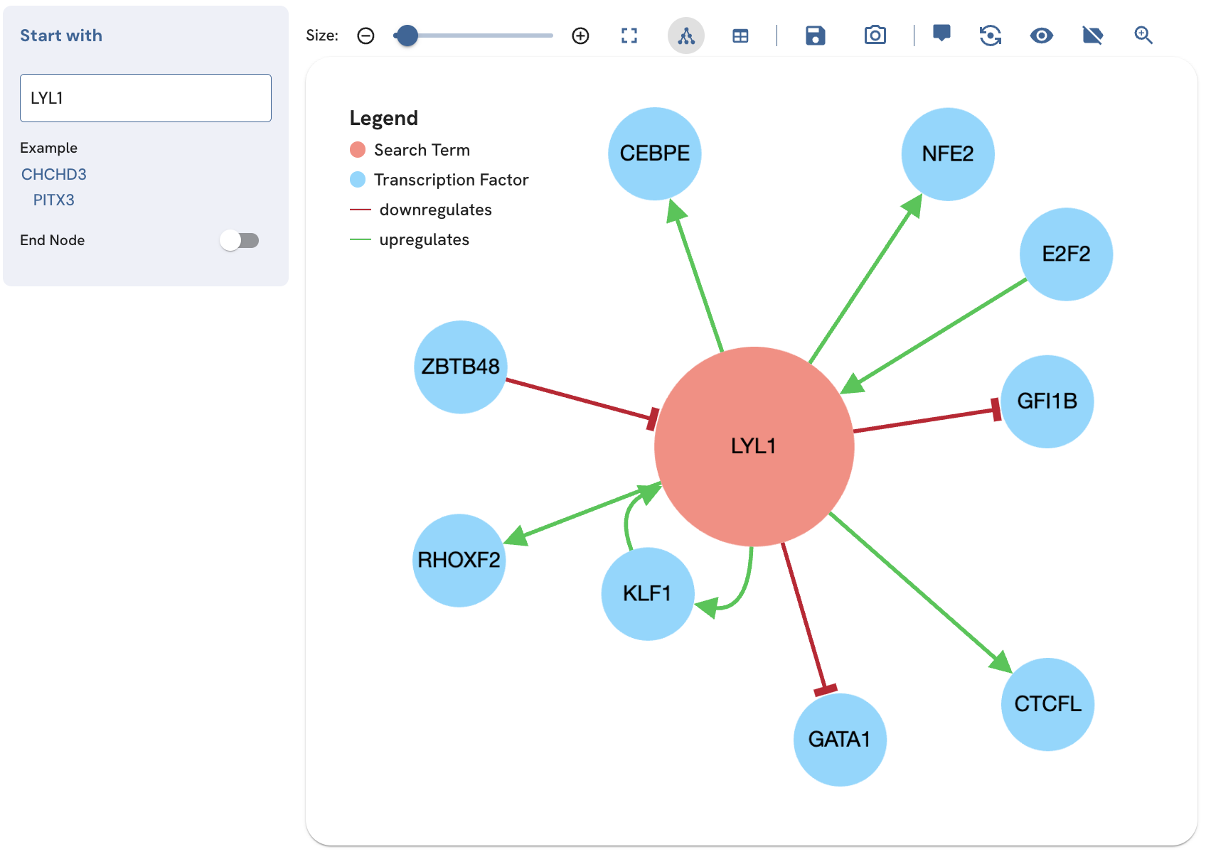
Fig. 13. Showing and adjusting the size of the legend.

Downloading the subnetwork

There are two methods for saving the subnetwork: saving the subnetwork as a file, or saving the subnetwork as an image.
Saving the subnetwork as a file produces two files:
      1 - nodes.csv has the fields [id, label, kind, uri, color]
      2 - edges.csv has the fields [source, target, relation, source_label, target_label, kind, p_value, z_score]

 

Saving the subnetwork as an image can be achieved by clicking on the camera icon. The subnetwork can be saved in PNG, JPEG, or SVG formats.

 

Enrichment Analysis with ChEA-KG

The enrichment analysis page provides the option to input a gene set for TF enrichment analysis with ChEA3 (Fig. 14). The enrichment analysis results are visualized as a ChEA-KG subnetwork connecting the enriched TFs.

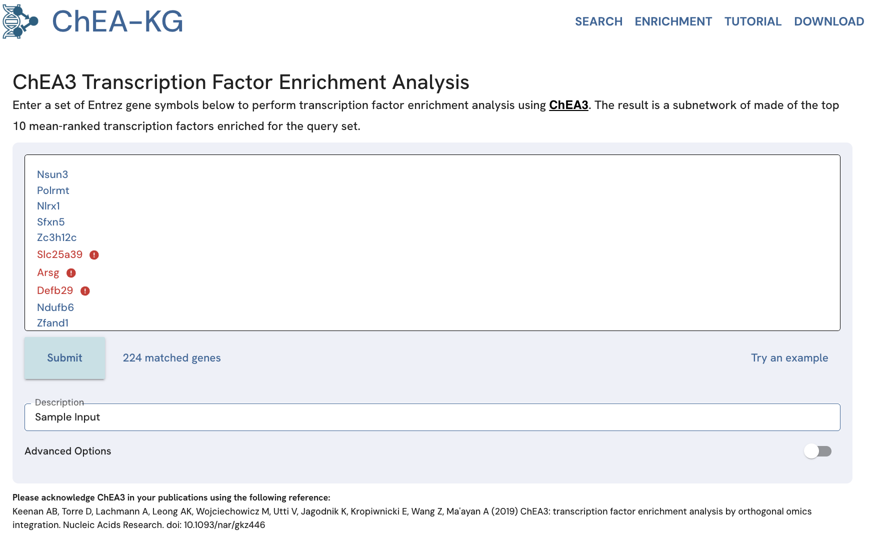
Fig. 14. The "Enrichment" tab landing page provides a textbox for inputting sets of human or mouse genes for TF enrichment analysis with ChEA3.

This feature generates a subnetwork made of the returned enriched TFs with the highest integrated Mean Rank scores for that input gene set. By default, the top 10 ranked TFs that appear in at least 3 out of 6 ChEA3 primary libraries are included. The ChEA3 integrated Mean Rank score is calculated by averaging the ranks from performing TF enrichment analysis against these 6 gene set libraries: Enrichr queries, GTEx co-expression, ARCHS4 co-expression, ENCODE ChIP-seq, Literature ChIP-seq, and ReMap ChIP-seq. For more information about the ChEA3 and the Mean Rank method, please refer to the ChEA3 publication.

NOTE: There are approximately 60 TFs cataloged by ChEA3 that are not included in the ChEA-KG GRN. This means that the subnetworks generated by this feature of ChEA-KG may contain fewer than the specified TFs.

Performing a gene set query

To perform a query, input a set of newline-separated Entrez gene symbols into the textbox. The submitted genes are automatically checked for valid Entrez gene symbols, and invalid gene symbols are flagged. Adding a description under the "Description" field is optional. Clicking "Submit" will invoke the ChEA3 enrichment analysis using the ChEA3 API.
To use an example gene set, click the "Try an example" link (Fig. 15).

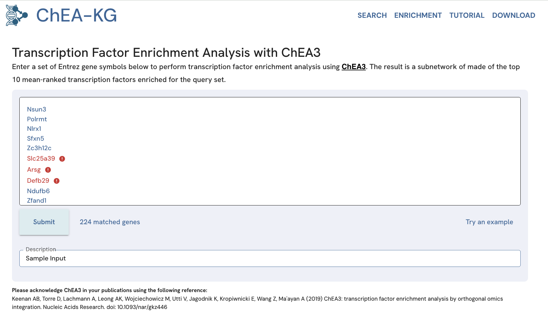
Fig. 15. Performing a ChEA3 query in ChEA-KG using the example gene set.

Clicking the "Submit" button should produce a TF subnetwork (Fig. 16). The toolbar at the top contains options to reformat and interact with the subnetwork. New queries can be performed using the form on the left.

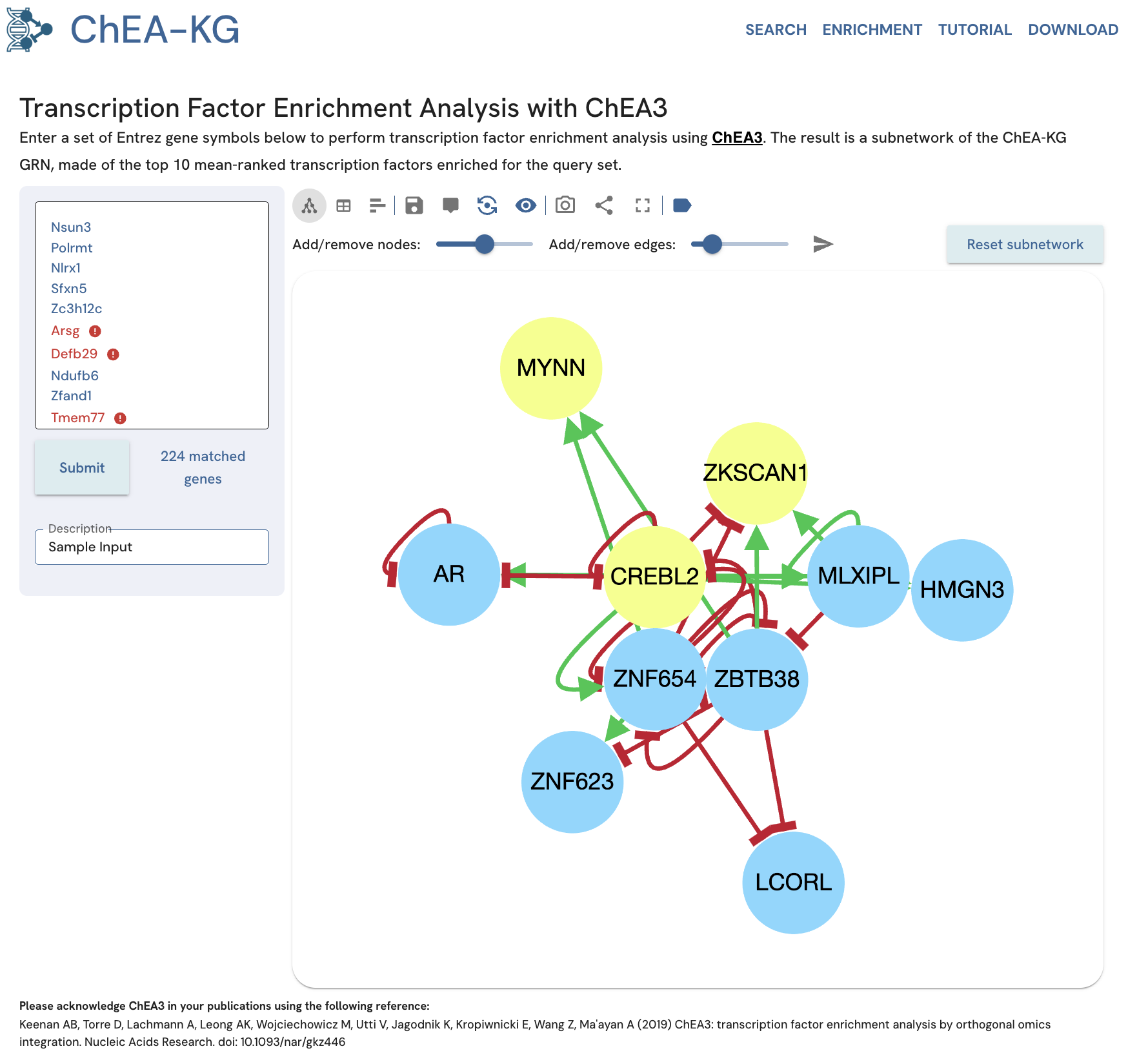
Fig. 16. Subnetwork of enriched TFs for an example gene set. Yellow nodes are enriched TFs that are also present in the input gene set.

Example dataset preparation:

To learn more about how to prepare your own dataset for submission to ChEA-KG enrichment, we developed two example workflows in Google Colab:

Both of these examples also show how to use the ChEA-KG API to access subnetwork data and visualize the subnetworks in Jupyter notebook.

Filtering the results and add more nodes and edges

The initial query results can be adjusted by adding and removing nodes and edges. Using the two sliders above the network view users can "add/remove nodes" by changing the number of nodes returned from the ChEA3 enrichment analysis. The slide provides the option to select 5-25 enriched TFs. Adjusting the z-score slider can be used to add/remove edges based on a Z score cutoff. These Z scores are not related to the enrichment analysis, but are from the original construction of the KG. To reset the subnetwork to the original settings, click "Reset subnetwork".

Example Adjust "Add/remove nodes" to 15 and click the send icon ("Submit changes"). The subnetwork will display the top 15 TFs for the same input gene set (Fig. 17).

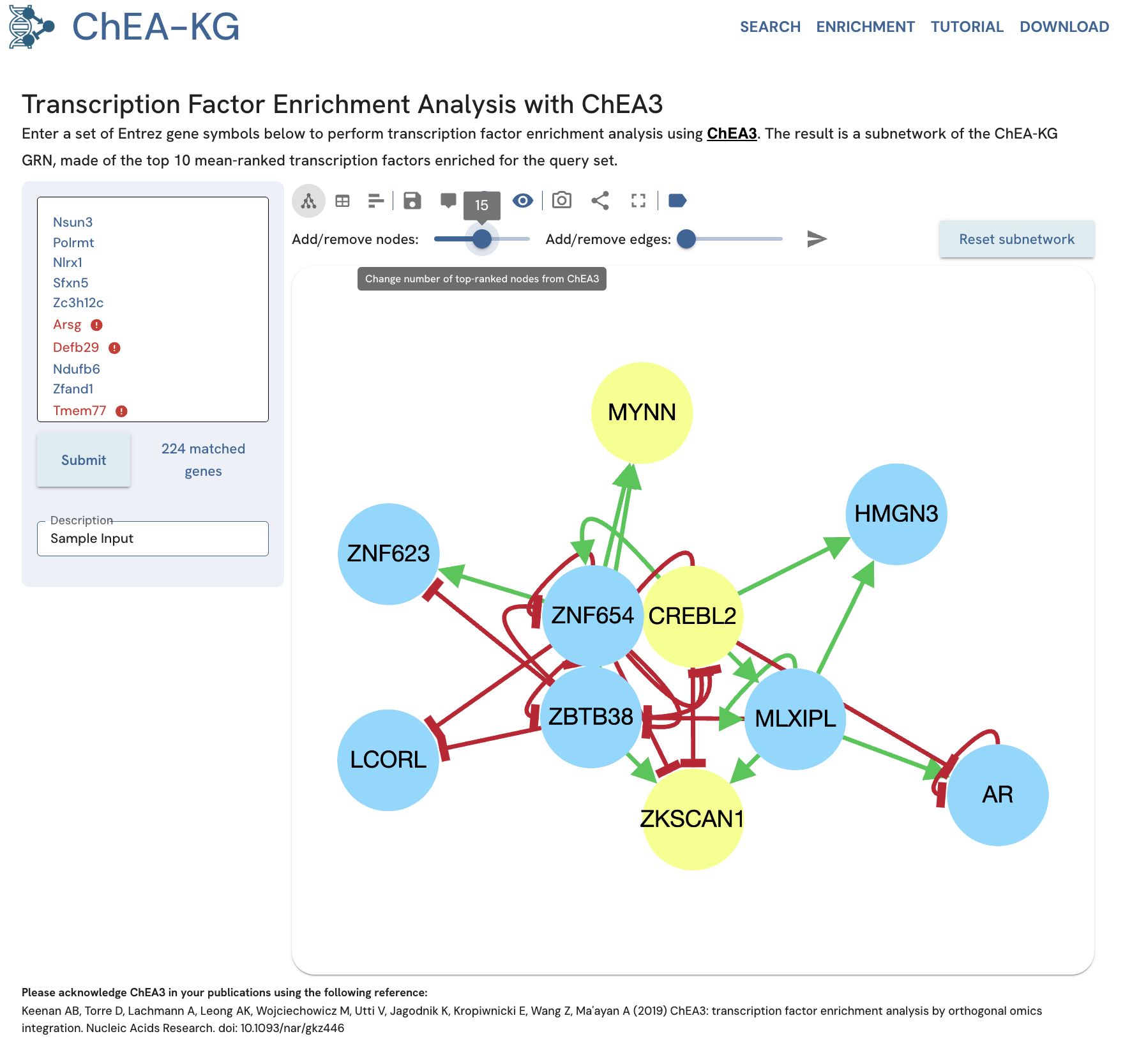
Fig. 17A. Changing the “Add TFs” to 15 can be used to increase the subnetwork size.

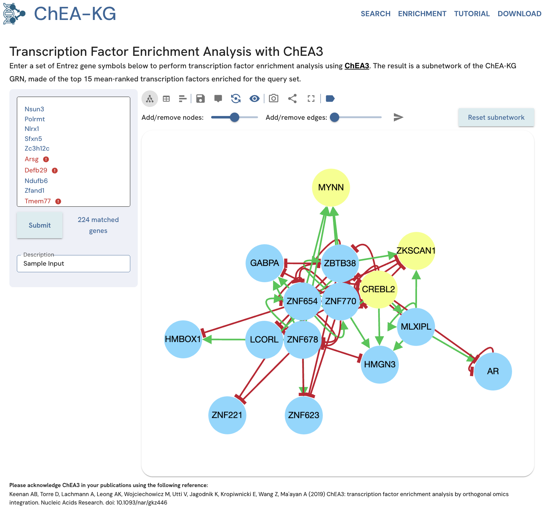
Fig. 17B. The returned subnetwork displays the top 15 nodes.

To change the number of edges, use the "Add/remove edges" slider to add/remove edges based on their Z score. The subnetwork will have the same number of TFs but more or less edges. Only TFs with edges that meet the specified threshold are kept (Fig. 18).

Fig. 18A. Filtering out edges with a Z score of less than 10 by adjusting the edges slider.

Fig. 18B. The network contains only TFs connected with edges that meet the new threshold.

Viewing the results as a table or a bar chart

The table view of the enrichment analysis results in ChEA-KG lists the enriched TFs, whether they also exist in the input gene set, the TF URI, the enrichment score, and the number of overlapping genes between the TF targets in ChEA3 and the genes from the input set (Fig. 19). The score indicates how relevant the gene set is for the enriched TF, with a lower score indicating more relevancy (higher average rank). The bar chart view displays the enriched TFs ordered by their score. Mousing over each bar displays a tooltip with the score and number of overlapping genes for that TF (Fig. 20).

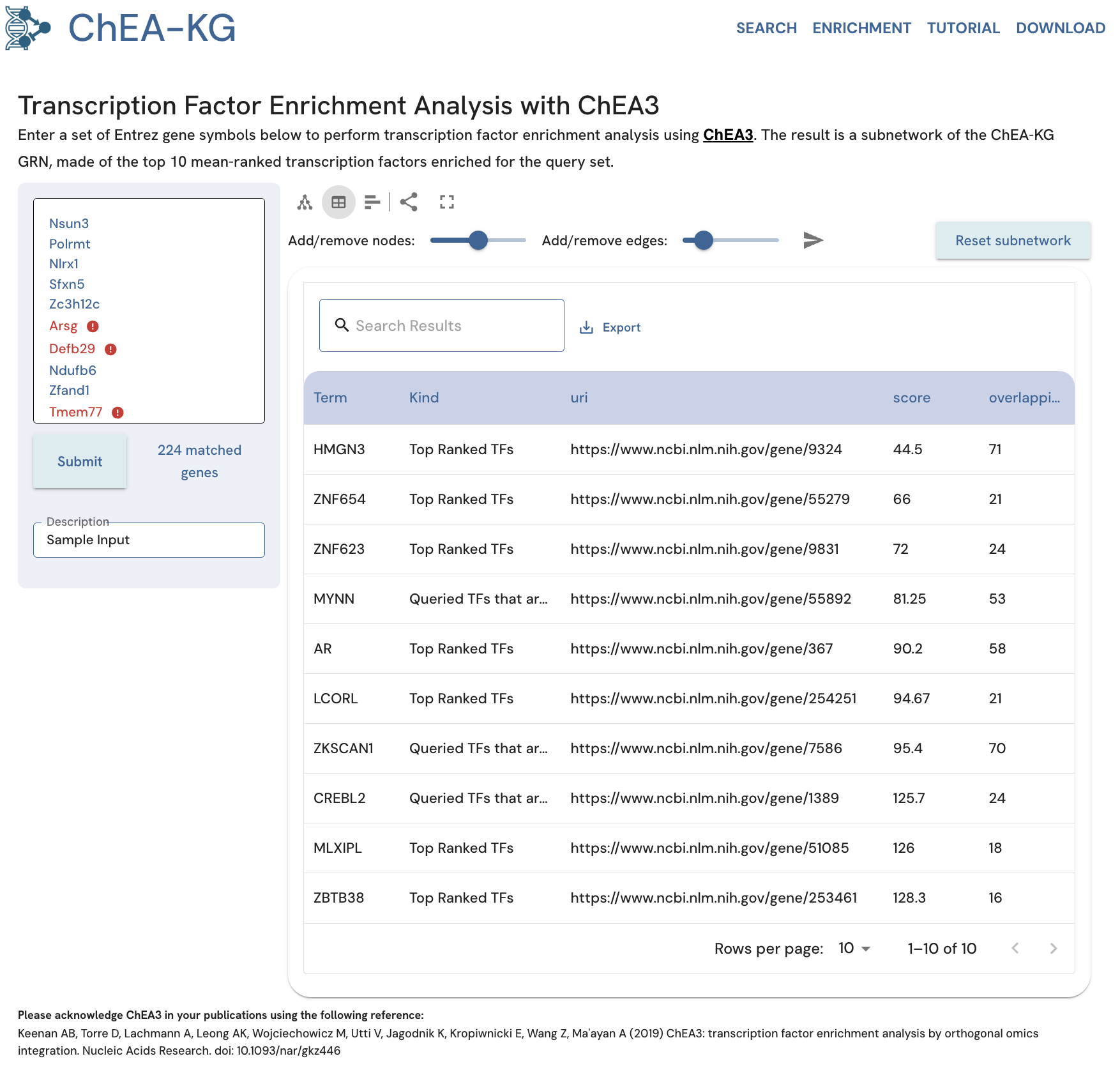
Fig. 19. View the ChEA-KG enrichment analysis results as a table.

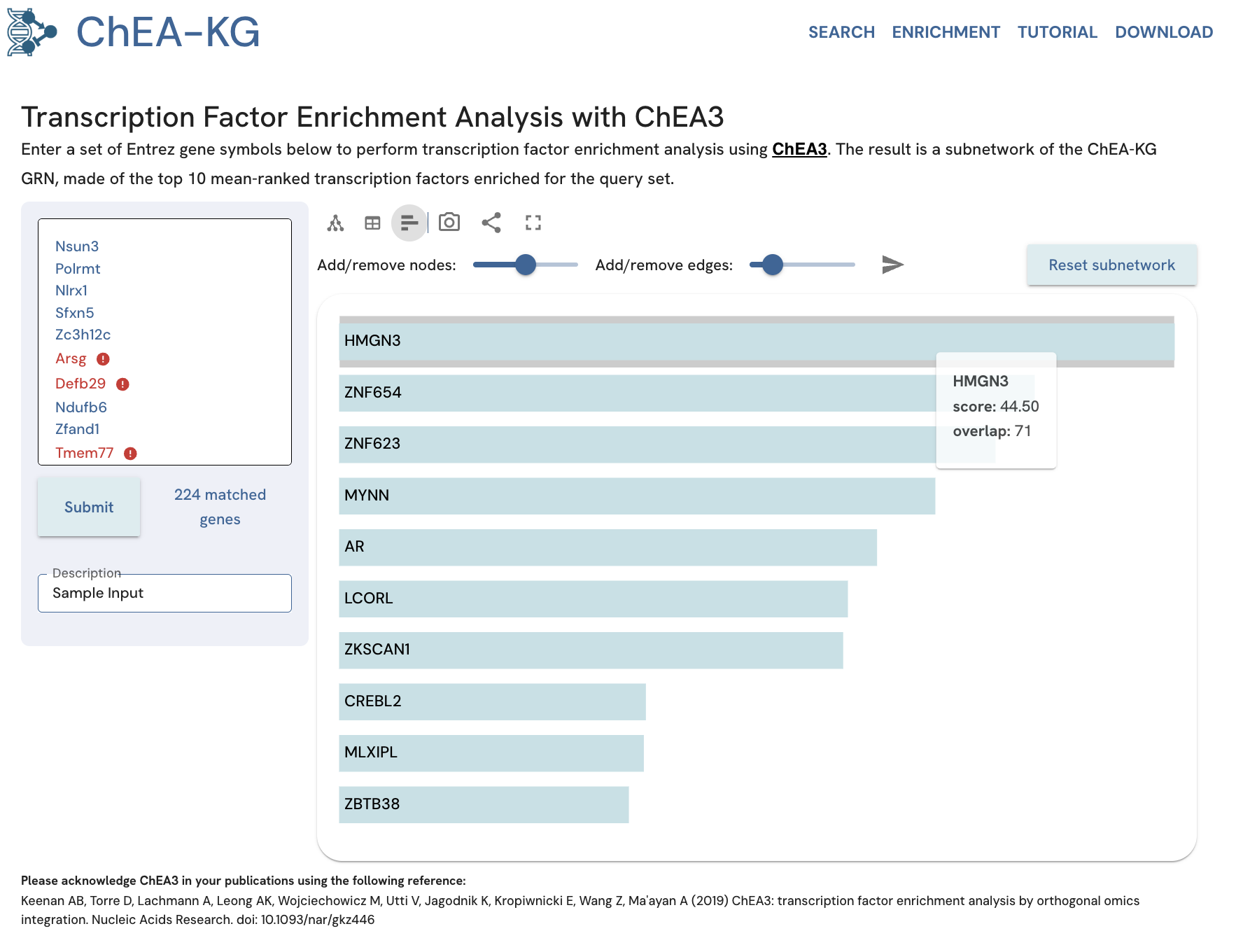
Fig. 20. View the ChEA-KG enrichment analysis results as a bar chart.

User Data

User-submitted gene sets are stored as unique node entities in the Neo4j database and are identified with a UUID that is produced when the set is originally submitted. This UUID is made part of the URL that provides permanent access to the results page of the submitted set. The UUID is kept private unless the user shares the URL with their colleagues. As the owners of the site, we guarantee that we have no intention to ever share, sell, analyze, post, or combine the uploaded gene sets with other users, and we will do our best effort to ensure that the database that stores these gene sets is secured.

API Documentation

The ChEA-KG API enables users to programmatically access the enrichment analysis feature. For more examples on how to use these endpoints, we have created two notebooks that show how to prepare and analyze gene sets with ChEA-KG, using either gene counts or BED files as input.

Analyze gene set

Method POST
URL /enrichment/addList
Returns JSON object with unique ID to view analysis results
Parameters

Example code:

CHEA_KG = 'https://chea-kg.maayanlab.cloud/api/enrichment'

gene_list = [MIR4454','RNU86','SNORD34','EEF1A1','RPL11','DCT','RPL37A','SNORD33','GAPDH','SNORD74','MIR4461','MIR4680','CD63','SNORD68',
'LDHA','TMSB4X','RPL27','SNORD108','MIR3191','RPS18','RPL41','ENO1','CAPG','RPS15A','SNORD79','FN1','LGALS3','GPNMB','NPM1','RPL7',
'RPS14','SNORD38A','RPS13','RPS7','ATOX1','PKM2','RPL31','SNORD76','SNORD42B','RPS29','BCYRN1','RPL6','ATP5E','RPS3A','RPL39','YWHAZ',
'TOMM7','RPS27A','SNORD49A','MIR4482-1','SNORD5','RPL30','MIR1292','RPL5','SNORD59A','RPS21','PSAP','RPL35A','RPL13AP5','SNORD50B',
'H2AFZ','SNORD27','PPIA','PRDX1','RPL21P28','RPL9','RPS12','HSP90B1','COX7C','RPL23','SNORD30','LDHB','GNB2L1','SGK1','FKBP1A','SNORD57',
'HSPD1','SNORD12','MIR4273','RPS4X','UQCRH','RPS2','COX5B','ATP5B','MIR4687','MIR4263','RPS10','RAN','MIR3687','PTTG1','SNORD87','ATP1A1',
'NME2','SNORD18A','RPSA','TUBB','RPL22','RPLP0','SNORD101','ANXA5','CD74','RPS6','MIR4691','GNAS','GSTO1','EIF4A1','NQO1','SNAR-G1',
'MIR4653','UBB','RPL38','SNORD4A','SNORD82','MIA','SNORD37','EIF3E','MIR4678','PDIA6','SLC25A3','PARK7','PGK1','C17orf76-AS1','YBX1',
'NCL','RPL35','HSP90AB1','MIR103B2','RPL26','DSTN','SNHG8','CALR','EEF1G','ATP5J2','TUBA1B','CSTB','SPP1','CALU','PABPC1','PRAME','LY6E',
'HNRNPA2B1','SNORD38B','SLC25A5','FABP5','MIR1915','SERPINF1','RPS8','DDOST','HINT1','RPL18A','RPS20','PSMA7','CHCHD2','HNRNPA1','RPL15',
'PSMA1','HLA-DRA','RPS3','RPL27A','EEF1B2','TXN','RPL4','SNORD16','PRNP','MDH1','NME1','CANX','SNORD35B','TBCA','TPI1','LOC645591','PTMA',
'ATP5A1','CBX3','SDCBP','C1QBP','DBI','SNORD59B','PLA1A','RPL37','NACA','CDK2','MIR324','RPS9','ALDOA','COX6A1','RPN2','ATP5F1','ATP5G3',
'SNAR-E','GMPR','SNRPD2','MIR4700','GYPC','CTSK','SHFM1','P4HB','CTSZ','MIR1260B','PCNA','HMGB1','COX7B','TM4SF1','SNORA41','CTSB',
'SLC20A1','IER3','ACSL3','CKS2','ATP1B3','MIR3188','ZNFX1-AS1','COX7A2','MIR135A1','PTGES3','CSDE1','LAMP2','SDC3','AMD1','MIR4523',
'SPON2','RPL10A','MIR4639','MIR4517','XRCC6','CSE1L','RPL8','MIR3653','MIR3190','SNORD54','RPL14','NBL1','ACTR3','ATP5C1','SNORD22',
'ATP1A1OS','EIF5A','SNORA10','GNG12','EIF3L','YWHAE','VDAC1','CD109','SRP9','ATP5H','SLIRP','MFI2','RPL19','LPXN','CLIC4','BTF3','HLA-A',
'FAM167B','PDIA3','SEC61G','MGST1','TXNRD1','ATP5G1','LITAF','HSD17B12','IVNS1ABP','SNORD31','NT5E','A2M','UBA52','POMP','HMGN2',
'ARL6IP5','HSP90AA1','SIRPA','EMP3','WFDC1','EIF3D','PYGB','SSBP1','SNRPB','RPL32','CCT7','IFI6','MCAM','RPL10','XRCC5','ATP6V1E1',
'SNRPG','MITF','RPL13A','MIR2861','C3orf14','C14orf2','RPS5','FBXO7','SPARC','SYPL1','RGS10','SLC45A2','APP','ANXA1','CD68','CCT2','IPO7',
'CCT4','HNRNPA3','CAP1','HSPE1','MBP','ACTR2','UCN2','MIR25','CASP1','EIF3I','SMS','MME','ARPC2','CDC42','NDUFB9','AP1S2','PRDX3','SRPX',
'PHGDH','FBL','CTSC','SNORA20','HNRNPH1','PDIA4','EIF3H','SOAT1','VGF','GANAB','HSPA9','GLO1','PRKAR1A','SNRPF','SDHB','TIMP1','PSMD6',
'BCL2A1','SNRPB2','NDUFB3','SNHG6','CORO1C','THOC7','SNX10','CEACAM1','LAPTM4B','SFRP1','ARPC3','G3BP1','COX17','GPM6B','SSR3','ETFB',
'MIR4665','CCT8','SLC43A3','GJB1','EIF4B','RPL18','KPNA2','CAPZB','FABP7','NOP56','HNRNPK','ERP29','VAMP8','OAT','PSMB1','CTSH','NSA2',
'LGALS3BP','SSB','LUZP6','POLE4','TIMP3','SF3B14','SUMO1','UGP2','PSMA2','PEG10','ERGIC3','ERH','MIR4785','C19orf79','PLP2','AKR1B1',
'AZIN1','RAB38','ADSL]

description = "Genes bound by AR in CCS1477-treated pancreatic cancer cells"

payload = {
    'list': (None, "\n".join(gene_list)),
    'description': (None, description)
}

response=requests.post(f"{CHEA_KG}/addList", files=payload)
data = json.loads(response.text)
print(data)

Example results

{'userListId': '4793eb83-6b01-4387-ac2b-15bc3f911cf3'}

View added gene set

Method GET
URL /enrichment/view
Returns JSON object with genes and description
Parameters

Example code:

response = requests.get(f'{CHEA_KG}/view?userListId={data['userListId']}')
if not response.ok:
    raise Exception('Error getting gene list')
    
data = json.loads(response.text)
print(data)

Example result:

{
    'set': ['PHF14', 'RBM3', 'MSL1', 'PHF21A', 'ARL10', 'INSR', 'JADE2', 'P2RX7', 'LINC00662', 'CCDC101', 
            'PPM1B', 'KANSL1L', 'CRYZL1', 'ANAPC16', 'TMCC1', 'CDH8', 'RBM11', 'CNPY2', 'HSPA1L', 'CUL2', 'PLBD2', 
            'LARP7', 'TECPR2', 'ZNF302', 'CUX1', 'MOB2', 'CYTH2', 'SEC22C', 'EIF4E3', 'ROBO2', 'ADAMTS9-AS2', 
            'CXXC1', 'LINC01314', 'ATF7', 'ATP5F1'], 
    'desc': 'Genes bound by AR in CCS1477-treated pancreatic cancer cells'
}

View enriched subnetwork data

Method GET
URL /enrichment/
Returns JSON formatted node and edge data
Parameters

Example code:

q = {
    'min_lib': 3, # minimum number of libraries that a TF must be ranked in
    'libraries': [
        {'library': "Integrated--meanRank", 'term_limit': 10} # edit term_limit to change number of top-ranked TFs
    ],
    'limit':50, # controls number of edges returned - may cause issues with visualization if too large
    'userListId': data['userListId']
}

query_json=json.dumps(q)

res = requests.post(CHEA_KG, data=query_json)
if res.ok:
    data = json.loads(res.text)
    print(data)
else:
    data = None
    print(res.text)

Example results:

{
	"nodes": [
		{
			"data": {
				"id": 7701,
				"kind": "Top Ranked TFs",
				"label": "ZNF142",
				"HGNC": "HGNC:12927",
				"Ensembl": "ENSG00000115568",
				"uri": "https://www.ncbi.nlm.nih.gov/gene/7701",
				"library": "Integrated--meanRank",
				"enrichr_label": "ZNF142",
				"score": 107,
				"rank": "7",
				"overlap": 3,
				"libs": [
					{
						"library": "ARCHS4 Coexpression",
						"score": 193
					},
					{
						"library": "Enrichr Queries",
						"score": 95
					},
					{
						"library": "GTEx Coexpression",
						"score": 33
					}
				],
				"rank_sum": 321,
				"value": 0.4604951343720062,
				"node_type": 0,
				"borderWidth": 0,
				"gradient_color": "#8ad6ff",
				"color": "#8ad6ff"
			}
		},
        ...
    ],
    [
        "edges": [
		{
			"data": {
				"source": 6664,
				"target": 6664,
				"source_label": "SOX11",
				"target_label": "SOX11",
				"kind": "Relation",
				"label": "downregulates",
				"p_value": 0,
				"z_score": 27.88027928302959,
				"relation": "downregulates",
				"lineColor": "#c70a2d",
				"directed": "tee"
			}
		},
        ...
        ]
    ]
}